Week 9 · Structure Analysis · Self-Similarity Matrices • compmus

Set-up

library(tidyverse)

## ── Attaching packages ─────────────────────────────────────── tidyverse 1.3.2 ──
## ✔ ggplot2 3.4.1     ✔ purrr   1.0.1
## ✔ tibble  3.1.8     ✔ dplyr   1.1.0
## ✔ tidyr   1.3.0     ✔ stringr 1.5.0
## ✔ readr   2.1.4     ✔ forcats 1.0.0
## ── Conflicts ────────────────────────────────────────── tidyverse_conflicts() ──
## ✖ dplyr::filter() masks stats::filter()
## ✖ dplyr::lag()    masks stats::lag()

library(spotifyr)
library(compmus)

In order for the code below to run, it is also necessary to set up Spotify login credentials for spotifyr.

New functions

Last week, we used several custom functions to work with the Spotify API:

get_tidy_audio_analysis to load audio analyses from Spotify, one track at a time
compmus_normalise to normalise audio features using common techniques, including:
- manhattan
- euclidean
- chebyshev
compmus_long_distance to compare to series of audio features against each other using common distance metrics, including:
- manhattan
- aitchison
- euclidean
- cosine
- angular

This week, we have a few new custom functions.

compmus_align aligns two levels of structure with each other, e.g., Spotify segments with beats or bars.
compmus_summarise helps to summarise features within higher levels of structure, including:
- mean
- acentre [Aitchison centre]
- rms [root mean square]
- max

Common combinations

Domain	Normalisation	Distance	Summary Statistic
Non-negative (e.g., chroma)	Manhattan	Manhattan	mean
		Aitchison	Aitchison centre
	Euclidean	cosine	root mean square
		angular	root mean square
	Chebyshev	[none]	max
Full-range (e.g., timbre)	[none]	Euclidean	mean
	Euclidean	cosine	root mean square
		angular	root mean square

Bloed, Zweet en Tranen

The following examples from Andre Hazes’s ‘Bloed, Zweet en Tranen’ highlight how to use these functions. Can you choose better combinations of normalisations, distances, and summary statistics?

bzt <- 
    get_tidy_audio_analysis('5ZLkc5RY1NM4FtGWEd6HOE') %>% 
    compmus_align(bars, segments) %>% 
    select(bars) %>% unnest(bars) %>% 
    mutate(
        pitches = 
            map(segments, 
                compmus_summarise, pitches, 
                method = 'rms', norm = 'euclidean')) %>% 
    mutate(
        timbre = 
            map(segments, 
                compmus_summarise, timbre, 
                method = 'mean'))

Cepstrogram

We can use compmus_gather_timbre much like compmus_gather_chroma last week to yield a cepstrogram. Try different levels of structure – Spotify’s estimates of beats, bars, or sections – to see which level is the most meaningful.

bzt %>% 
    compmus_gather_timbre %>% 
    ggplot(
        aes(
            x = start + duration / 2, 
            width = duration, 
            y = basis, 
            fill = value)) + 
    geom_tile() +
    labs(x = 'Time (s)', y = NULL, fill = 'Magnitude') +
    scale_fill_viridis_c(option = 'E') +
    theme_classic()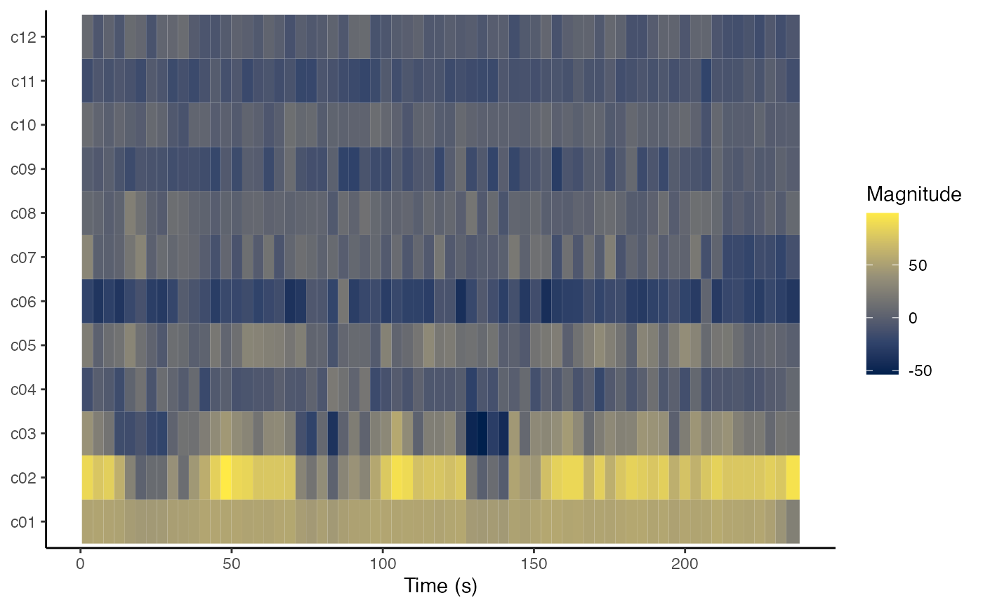

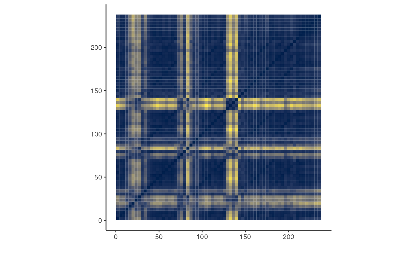
Self-Similarity Matrices

The function compmus_self_similarity is a wrapper around compmus_long_distance from last week, for the case where the distances are computed form the same track. Try different distance functions to see what is most useful for this track – and compare your results with a self-similarity matrix based on chroma.

bzt %>% 
    compmus_self_similarity(timbre, 'cosine') %>% 
    ggplot(
        aes(
            x = xstart + xduration / 2, 
            width = xduration,
            y = ystart + yduration / 2,
            height = yduration,
            fill = d)) + 
    geom_tile() +
    coord_fixed() +
    scale_fill_viridis_c(option = 'E', guide = 'none') +
    theme_classic() +
    labs(x = '', y = '')

Week 9 · Structure Analysis · Self-Similarity Matrices