Week 10 · Key and Chord Estimation
John Ashley Burgoyne
6 March 2019
compmus-w10.RmdSet-up
## ── Attaching packages ─────────────────────────────────────── tidyverse 1.3.2 ──
## ✔ ggplot2 3.4.1     ✔ purrr   1.0.1
## ✔ tibble  3.1.8     ✔ dplyr   1.1.0
## ✔ tidyr   1.3.0     ✔ stringr 1.5.0
## ✔ readr   2.1.4     ✔ forcats 1.0.0
## ── Conflicts ────────────────────────────────────────── tidyverse_conflicts() ──
## ✖ dplyr::filter() masks stats::filter()
## ✖ dplyr::lag() masks stats::lag()In order for the code below to run, it is also necessary to set up
Spotify login credentials for spotifyr.
Tonal Templates
The focus of the readings this week were chord and key estimation. One set of standard templates is below: 1–0 coding for the chord templates and the Krumhansl–Kessler key profiles.
circshift <- function(v, n) {if (n == 0) v else c(tail(v, n), head(v, -n))}

    # C     C#    D     Eb    E     F     F#    G     Ab    A     Bb    B
major_chord <-
    c(1,    0,    0,    0,    1,    0,    0,    1,    0,    0,    0,    0)
minor_chord <-
    c(1,    0,    0,    1,    0,    0,    0,    1,    0,    0,    0,    0)
seventh_chord <-
    c(1,    0,    0,    0,    1,    0,    0,    1,    0,    0,    1,    0)

major_key <-
    c(6.35, 2.23, 3.48, 2.33, 4.38, 4.09, 2.52, 5.19, 2.39, 3.66, 2.29, 2.88)
minor_key <-
    c(6.33, 2.68, 3.52, 5.38, 2.60, 3.53, 2.54, 4.75, 3.98, 2.69, 3.34, 3.17)

chord_templates <-
    tribble(
        ~name  , ~template,
        'Gb:7'  , circshift(seventh_chord,  6),
        'Gb:maj', circshift(major_chord,    6),
        'Bb:min', circshift(minor_chord,   10),
        'Db:maj', circshift(major_chord,    1),
        'F:min' , circshift(minor_chord,    5),
        'Ab:7'  , circshift(seventh_chord,  8),
        'Ab:maj', circshift(major_chord,    8),
        'C:min' , circshift(minor_chord,    0),
        'Eb:7'  , circshift(seventh_chord,  3),
        'Eb:maj', circshift(major_chord,    3),
        'G:min' , circshift(minor_chord,    7),
        'Bb:7'  , circshift(seventh_chord, 10),
        'Bb:maj', circshift(major_chord,   10),
        'D:min' , circshift(minor_chord,    2),
        'F:7'   , circshift(seventh_chord,  5),
        'F:maj' , circshift(major_chord,    5),
        'A:min' , circshift(minor_chord,    9),
        'C:7'   , circshift(seventh_chord,  0),
        'C:maj' , circshift(major_chord,    0),
        'E:min' , circshift(minor_chord,    4),
        'G:7'   , circshift(seventh_chord,  7),
        'G:maj' , circshift(major_chord,    7),
        'B:min' , circshift(minor_chord,   11),
        'D:7'   , circshift(seventh_chord,  2),
        'D:maj' , circshift(major_chord,    2),
        'F#:min', circshift(minor_chord,    6),
        'A:7'   , circshift(seventh_chord,  9),
        'A:maj' , circshift(major_chord,    9),
        'C#:min', circshift(minor_chord,    1),
        'E:7'   , circshift(seventh_chord,  4),
        'E:maj' , circshift(major_chord,    4),
        'G#:min', circshift(minor_chord,    8),
        'B:7'   , circshift(seventh_chord, 11),
        'B:maj' , circshift(major_chord,   11),
        'D#:min', circshift(minor_chord,    3),
)

key_templates <-
    tribble(
        ~name    , ~template,
        'Gb:maj', circshift(major_key,  6),
        'Bb:min', circshift(minor_key, 10),
        'Db:maj', circshift(major_key,  1),
        'F:min' , circshift(minor_key,  5),
        'Ab:maj', circshift(major_key,  8),
        'C:min' , circshift(minor_key,  0),
        'Eb:maj', circshift(major_key,  3),
        'G:min' , circshift(minor_key,  7),
        'Bb:maj', circshift(major_key, 10),
        'D:min' , circshift(minor_key,  2),
        'F:maj' , circshift(major_key,  5),
        'A:min' , circshift(minor_key,  9),
        'C:maj' , circshift(major_key,  0),
        'E:min' , circshift(minor_key,  4),
        'G:maj' , circshift(major_key,  7),
        'B:min' , circshift(minor_key, 11),
        'D:maj' , circshift(major_key,  2),
        'F#:min', circshift(minor_key,  6),
        'A:maj' , circshift(major_key,  9),
        'C#:min', circshift(minor_key,  1),
        'E:maj' , circshift(major_key,  4),
        'G#:min', circshift(minor_key,  8),
        'B:maj' , circshift(major_key, 11),
        'D#:min', circshift(minor_key,  3))
Chordograms and Keygrams
Armed with these templates, we can make chordograms and keygrams for
individual pieces. Similar to previous weeks, we start by choosing a
level of hierarchy and then summarise the chroma features a that level.
Higher levels like section are more appropriate for key
profiles; lower levels like beat are more appropriate for
chord profiles.
The following code fetches the analysis for Zager and Evans’s ‘In the Year 2525’ (1969).
twenty_five <-
    get_tidy_audio_analysis('5UVsbUV0Kh033cqsZ5sLQi') %>%
    compmus_align(sections, segments) %>%
    select(sections) %>% unnest(sections) %>%
    mutate(
        pitches =
            map(segments,
                compmus_summarise, pitches,
                method = 'mean', norm = 'manhattan'))
The new helper function compmus_match_pitch_template
compares the averaged chroma vectors against templates to yield a
chordo- or keygram. The two truck-driver modulations from G-sharp minor
through A minor to B-flat minor are clear.
twenty_five %>%
    compmus_match_pitch_template(key_templates, 'euclidean', 'manhattan') %>%
    ggplot(
        aes(x = start + duration / 2, width = duration, y = name, fill = d)) +
    geom_tile() +
    scale_fill_viridis_c(option = 'E', guide = 'none') +
    theme_minimal() +
    labs(x = 'Time (s)', y = '')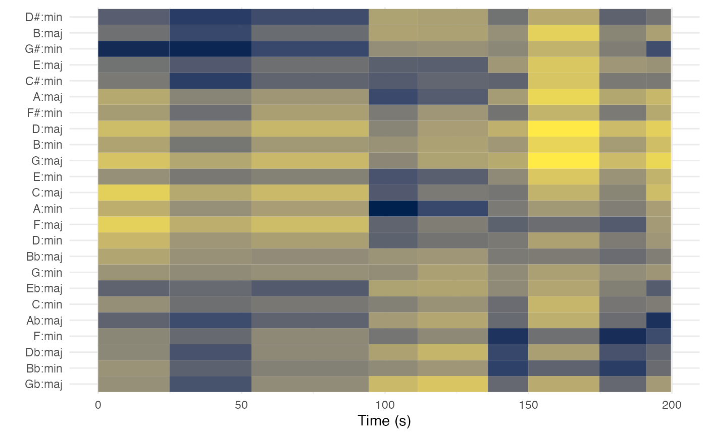
Once you have the code running, try the following adaptations.
- Try summarising the track at different levels of hierarchy (beats, bars, sections), as well as different combinations of summarisation methods and norms, just as previous weeks. The table below repeats the combinations we have considered.
- Try making a chordogram instead of the keygram above.
- Replace the key profiles above with Temperley’s proposed improvements from the reading this week. (Don’t forget to re-run the chunk after you are finished.) Do the revised profiles work any better? Can you think of a way to improve the chord profiles, too?
| Domain | Normalisation | Distance | Summary Statistic |
|---|---|---|---|
| Non-negative (e.g., chroma) | Manhattan | Manhattan | mean |
| Aitchison | Aitchison centre | ||
| Euclidean | cosine | root mean square | |
| angular | root mean square | ||
| Chebyshev | [none] | max | |
| Full-range (e.g., timbre) | [none] | Euclidean | mean |
| Euclidean | cosine | root mean square | |
| angular | root mean square |
Track-Level Summaries
Several students have asked how to incorporate the low-level audio analysis features at the playlist level. Here is one strategy for doing so, which we will extend next week. As an example, let’s consider the difference between Spotify’s ‘Sound of’ playlists for bebop and big band.
After loading the playlists, we can use the helper function
add_audio_analysis to fetch the low-level features for
every track. Adding audio analysis for every track is a slow operation,
and so for the purposes of this exercise, we will limit ourselves to 30
tracks from each playlist. The results makes heavy use of list-columns,
which are discussed in more detail in the optional purrr
exercise on DataCamp.
bebop <-
    get_playlist_audio_features(
        'thesoundsofspotify',
        '55s8gstHcaCyfU47mQgLrB') %>%
    slice(1:30) %>%
    add_audio_analysis()
bigband <-
    get_playlist_audio_features(
        'thesoundsofspotify',
        '2cjIvuw4VVOQSeUAZfNiqY') %>%
    slice(1:30) %>%
    add_audio_analysis()
jazz <-
    bebop %>% mutate(genre = "Bebop") %>%
    bind_rows(bigband %>% mutate(genre = "Big Band"))
For non-vector features, we can use the summarise_at
command to collect summary statistics like mean and standard
deviation.
jazz %>%
    mutate(
        sections =
            map(
                sections,
                summarise_at,
                vars(tempo, loudness, duration),
                list(section_mean = mean, section_sd = sd))) %>%
    unnest(sections) %>%
    ggplot(
        aes(
            x = tempo,
            y = tempo_section_sd,
            colour = genre,
            alpha = loudness)) +
    geom_point(aes(size = duration / 60)) +
    geom_rug() +
    theme_minimal() +
    ylim(0, 5) +
    labs(
        x = 'Mean Tempo (bpm)',
        y = 'SD Tempo',
        colour = 'Genre',
        size = 'Duration (min)',
        alpha = 'Volume (dBFS)')
## Warning: Removed 13 rows containing missing values (`geom_point()`).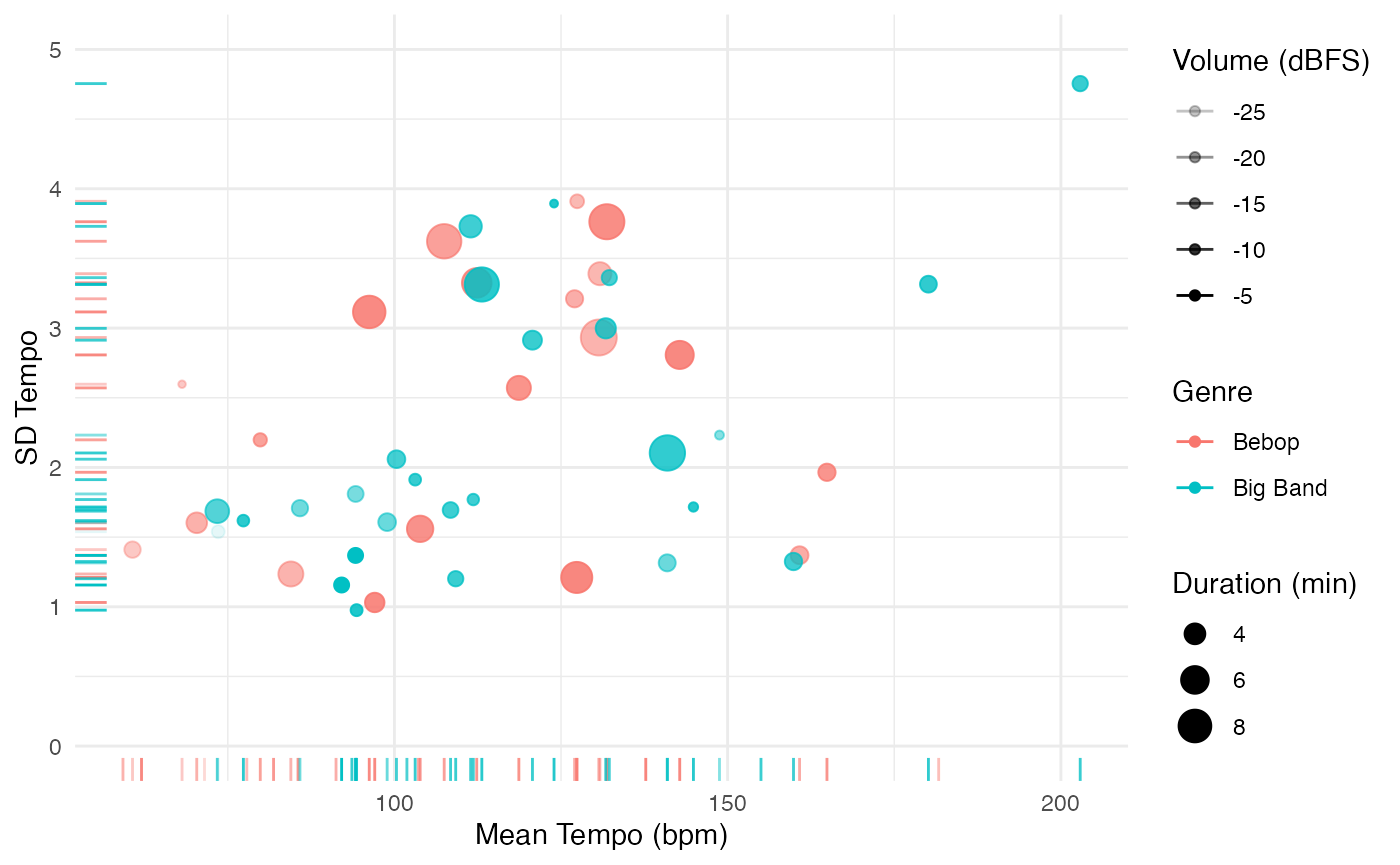
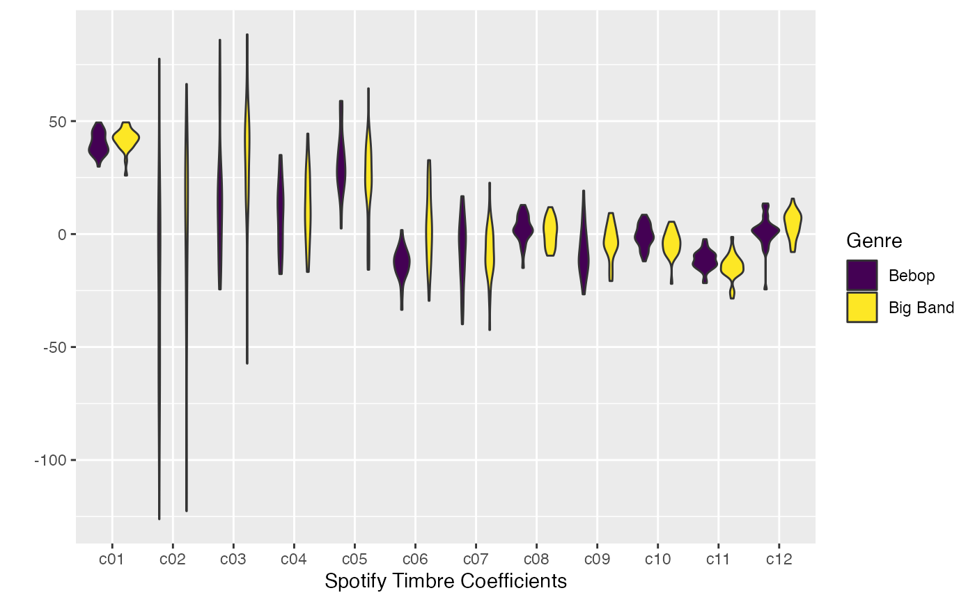
When working with vector-valued features like chroma or timbre, we need to use functions from the previous weeks. Here is an example of comparing average timbre coefficients in bebop and big band. Coefficient 6 looks like the most promising marker distinguishing these genres, but we should verify that with cepstrograms and listening tests of specific pieces, supported by the Spotify documentation for its timbre features.
jazz %>%
    mutate(
        timbre =
            map(
                segments,
                compmus_summarise,
                timbre,
                method = 'mean')) %>%
    select(genre, timbre) %>%
    compmus_gather_timbre %>%
    ggplot(aes(x = basis, y = value, fill = genre)) +
    geom_violin() +
    scale_fill_viridis_d() +
    labs(x = 'Spotify Timbre Coefficients', y = '', fill = 'Genre')